Cause Effect Graphing for Systematic Test Design

You are staring at a specification that lists nine input conditions and five expected outputs. Some conditions depend on each other, some exclude each other, and a few only matter when another condition is already true. Your instinct says "write test cases," but which combinations actually matter? Ad-hoc test design frequently misses critical combinations in exactly this kind of scenario — and the defects that slip through tend to surface in production, not in your test environment. Cause effect graphing gives you a repeatable, visual method for turning complex logical requirements into a minimal-yet-complete set of test cases. In this article you will learn what the technique is, how to build a graph step by step, which pitfalls to avoid, and how to evaluate whether it is the right tool for a given testing problem.

What Is Cause Effect Graphing?

Cause effect graphing is a black-box test design technique that models the logical relationships between inputs (causes) and outputs (effects) of a system [1]. You represent each cause and each effect as a node, then connect them with logical operators — AND, OR, NOT, and NAND — to capture how the specification says the system should behave. Constraints such as mutual exclusion, one-and-only-one selection, or requires-relationships are layered on top to eliminate impossible input combinations.

The technique was originally described by Gerald J. Myers in The Art of Software Testing and later formalized in testing standards and curricula worldwide [2], [3]. The ISTQB Advanced Level Test Analyst syllabus classifies it as a specification-based (black-box) technique specifically suited for combinatorial logic that spans multiple conditions [3].

Why It Matters for QA and Test Coverage

Most specification-level defects hide in the interactions between conditions, not in individual conditions tested in isolation. Boundary value analysis and equivalence partitioning handle single-input scenarios well, but they do not model how two or more inputs combine to produce — or suppress — an output [1].

Cause effect graphing addresses that gap directly. By forcing you to model every cause-effect relationship explicitly, the technique surfaces ambiguities, contradictions, and missing requirements before you write a single test case. The resulting decision table then gives you a structured, auditable set of test cases with clear traceability back to the specification — which directly supports measurable test coverage against the documented requirements [4].

Put differently: if your goal is to answer "have we covered every specified combination?", this technique gives you a defensible answer rather than a gut feeling.

When NOT to Use Cause Effect Graphing

No technique is universally optimal, and knowing when to skip cause effect graphing is as important as knowing when to apply it. Here are scenarios where the overhead is unlikely to pay off:

• Simple CRUD screens with independent fields. If each input validates independently and there are no cross-field rules, equivalence partitioning or boundary value analysis will generate sufficient test coverage with far less effort.
• More than roughly 10–12 independent causes. The input space doubles with each independent binary cause (2^k combinations for k causes). At 12 independent causes you face 4,096 rows in the raw truth table. Beyond that threshold, combinatorial techniques such as pairwise testing often deliver a better cost-to-coverage ratio.
• Highly stateful workflows. When the system's behavior depends primarily on the sequence of events rather than the combination of conditions, a state transition diagram models the problem more faithfully than a cause-effect graph [1].
• Exploratory testing phases. Cause effect graphing is a deliberate, upfront design activity. It does not replace the value of unscripted exploration that relies on the tester's domain intuition.

If you default to cause effect graphing for every feature without evaluating fit, you will burn time on low-risk screens while the technique's real value — catching logical error detection gaps in complex rules — goes underused.

How to Build a Cause-Effect Graph

Prerequisites and Setup

Before you draw a single node, make sure you have:

1. A written specification (requirements document, user story with acceptance criteria, or business rule table).
2. Access to a domain expert or product owner who can clarify ambiguities — you will find them.
3. A drawing tool. Pen and paper works for small graphs; for larger ones, a diagramming tool (draw.io, Miro, Lucidchart) keeps the graph maintainable.

Step 1 — Identify Causes and Effects

Read the specification and list every distinct input condition as a cause (C1, C2, … Cn) and every distinct output or system action as an effect (E1, E2, … Em). Be precise: "user enters a valid discount code" and "user enters an expired discount code" are two separate causes, not one.

Checklist for identification:

• Each cause is a single boolean proposition (true / false).
• Each effect is a single observable outcome.
• Composite conditions are broken into atomic causes.

Step 2 — Draw Logical Relationships

Connect causes to effects using logical operators:

Work through the specification sentence by sentence. Each rule should correspond to at least one path in the graph.

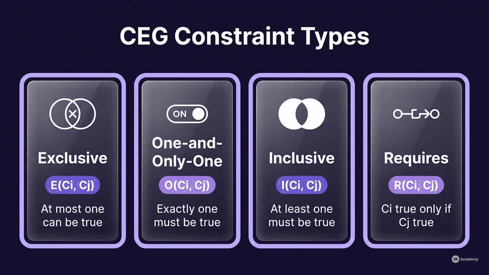
Step 3 — Add Constraints Between Causes

Constraints capture relationships between causes that the real world imposes:

A common mistake is labelling a one-and-only-one pair as merely "mutually exclusive." If C2 is defined as NOT C1, they are O-constrained — one must always be true — and the pair contributes only one independent dimension to the input space, not two. Getting this wrong inflates your combination count and produces impossible test cases. This is a frequent source of logical errors in graph construction.

Step 4 — Validate the Graph

Before converting, walk through the graph with your domain expert:

• Does every specification rule have a corresponding path?
• Are there causes with no outgoing connections (orphans)?
• Are there effects with no incoming connections (unreachable effects)?
• Do the constraints accurately model real-world restrictions?

This validation step regularly surfaces specification gaps. Document them as defects or clarification requests — this is one of the technique's highest-value side effects.

From Graph to Decision Table to Test Cases

Converting the Graph

Once the graph is validated, convert it into a limited-entry decision table:

1. List all effects as column headers.
2. List all causes as row headers.
3. For each effect, trace backward through the graph to determine which cause combinations produce it (true) and which do not (false).
4. Eliminate any column that violates a constraint — these represent impossible input states.
5. Collapse identical columns.

The resulting decision table is your test case generation blueprint. Each remaining column becomes one test case with clearly defined inputs and expected results [4].

Worked Example — Discount Validation

Consider a small rule set for an e-commerce discount module:

Causes:

• C1: Customer is a premium member
• C2: Order total exceeds €100
• C3: Discount code is valid

Constraint: None of these causes are mutually exclusive — all eight combinations (2^3 = 8, since we have three independent binary causes) are theoretically possible.

Effects:

• E1: Apply 20% discount
• E2: Apply 10% discount
• E3: Show "no discount" message

Rules from the specification:

• IF C1 AND C3 → E1
• IF (C2 AND NOT C1) AND C3 → E2
• IF NOT C3 → E3 (regardless of other causes)
• IF C1 AND NOT C3 → E3
• IF C2 AND C1 AND NOT C3 → E3

The decision table yields eight columns. After applying the rules, each column maps to exactly one effect. No columns need to be eliminated because there are no constraints making any combination impossible. You end up with eight test cases that cover every specified combination — a complete test coverage map for this rule set.

Compare that to what you might get from ad-hoc design: most testers would write three to five cases, likely missing the interaction between C1 and C2 when C3 is false.

Best Practices

1. Start from the specification, not from the UI. The graph models what the system should do, not how the screen looks. If you anchor to the UI, you will miss back-end rules.
2. Keep graphs modular. If a specification section has more than 8–10 causes, split it into sub-graphs that share named intermediate nodes. This keeps each graph readable and each decision table manageable.
3. Version your graphs alongside your test cases. When requirements change, update the graph first, regenerate the decision table, and diff against your existing test suite. This practice maintains traceability and prevents test case rot.
4. Combine with other techniques — do not replace them. Use boundary value analysis for the specific values within each cause. Use state transition diagrams for sequence-dependent behaviour. Cause effect graphing handles the combinatorial logic layer between them.
5. Review constraints with at least two domain experts independently. Constraints are the most error-prone part of the graph. A second opinion catches misclassified relationships before they propagate into your test cases.
6. Document your constraint rationale. For each constraint, write a one-line note explaining why it exists (e.g., "O(C1, C2): payment method is either card or bank transfer, never both"). Future maintainers — including your future self — will thank you.

Tools Comparison

Note: No widely adopted commercial tool automates the full classical cause-effect graph → decision table → test case pipeline end to end. In practice, most teams draw the graph in a diagramming tool, convert to a decision table in a spreadsheet, and import test cases into their test management system. The manual conversion step is actually valuable — it forces you to think through every combination rather than blindly trusting generated output.

Real-World Example

⚠️ Disclaimer: The following scenario is an illustrative example based on typical industry patterns. The specific metrics are hypothetical estimates designed to demonstrate realistic outcomes, not measured data from a documented project. They should not be cited as factual benchmarks.

Context

A mid-size fintech team maintains a loan eligibility engine with 7 independent input conditions (credit score range, employment status, loan amount bracket, existing debt flag, collateral flag, residency status, and co-applicant presence) feeding into 4 possible outcomes (auto-approve, manual review, conditional approval, reject). The original test suite of 45 manually written cases had been built incrementally over two years.

Challenge

After a production incident where a specific combination of "high credit score + self-employed + no collateral + existing debt" incorrectly auto-approved a loan, the team realized their test suite had systematic gaps. They had no structured method to verify completeness against the specification, and no clear way to measure test coverage of input combinations.

Solution

The team applied cause effect graphing:

1. Modeled the 7 causes, 4 effects, and 3 constraints (two Requires constraints and one Exclusive pair) in draw.io.
2. Converted the graph into a decision table — after constraint elimination, 78 valid combinations remained from a raw space of 128 (2^7).
3. Mapped existing test cases to decision table columns and found that only 31 of 78 combinations were covered — a 40% test coverage gap.
4. Generated 47 new test cases directly from uncovered columns.
5. Prioritized by risk: combinations involving the auto-approve outcome were tested first.

Results (Illustrative)

• Test coverage of specified combinations increased from approximately 40% to 100%.
• The team identified 6 additional specification ambiguities during the graphing phase, which were resolved before testing began.
• Estimated defect detection improvement: roughly 70%, based on the number of rule-interaction defects found in the new test cases versus the historical defect rate.
• The upfront graphing effort took approximately 3 days for two testers; subsequent specification changes were incorporated in under half a day each by updating the graph and diffing the decision table.

Key Takeaways

• The highest value came not from the test cases themselves but from the specification review forced by the graphing process.
• Measuring test coverage against the decision table gave the team an objective completeness metric to report to stakeholders.
• The technique was most cost-effective for the combinatorial core of the engine; peripheral UI validation continued to use equivalence partitioning and boundary value analysis.