



Your requirements document says "if the user is logged in and the account is active and the subscription is valid, grant access — unless the account is flagged." You read it twice. Three conditions, at least one exception, and you know a fourth condition is hiding somewhere in the acceptance criteria. If you try to test this from memory, you will miss combinations. If you write test cases one by one, you will duplicate some and skip others. A decision table gives you a systematic way to lay out every condition, map every rule combination, and trace each one to a specific action — so nothing slips through. This article walks you through building one from scratch, compares decision tables with related techniques, and shows you a practical workflow you can apply on your next sprint.
What Is a Decision Table?
A decision table is a structured grid that maps every relevant combination of input conditions to the actions (or outputs) the system should produce. The ISTQB Foundation Level syllabus defines decision table testing as a black-box test technique in which test cases are designed to exercise the combinations of conditions and resulting actions shown in a decision table [1]. ISO/IEC/IEEE 29119-4 further formalizes the technique as a method for deriving test cases from a specification of conditions and their corresponding actions [2].
The table has four quadrants:
Conditions | Actions | |
|---|---|---|
Stubs (labels) | Condition stubs — the names of each input or state (e.g., "Account active?") | Action stubs — the names of each possible system response (e.g., "Grant access") |
Entries (values) | Condition entries — True, False, or "—" (don't care) for each rule | Action entries — X (execute) or blank (skip) for each rule |
Each column of entries is a rule — one specific combination of conditions and the actions it triggers. If you have k independent binary conditions with no constraints, the full table contains 2^k rules.
Why Decision Tables Matter in QA
Three practical reasons keep decision tables relevant across projects:
Exhaustive coverage of business logic. When conditions interact — when Condition A changes the meaning of Condition B — isolated test cases miss the interplay. A decision table forces you to address every rule combination explicitly, so gaps become visible before execution.
Traceability to requirements. Each rule links directly to a business rule or acceptance criterion. During review, stakeholders can point at a column and say "this combination shouldn't trigger that action," giving you a feedback loop that is harder to achieve with unstructured test lists.
Efficient test reduction. Not every combination needs its own test case. Where the outcome is the same regardless of a condition's value, you collapse rules using "don't care" entries. According to the ISTQB syllabus, this simplification can substantially reduce the number of test cases while preserving the coverage of the underlying logic [1]. Lee Copeland's work on test design techniques describes the same principle — rules producing identical actions can be merged, reducing the table without sacrificing logical completeness [3].
How to Build a Decision Table Step by Step
Here is a repeatable workflow. You can apply it in a spreadsheet, a wiki page, or a dedicated test management tool.
Step 1 — Identify the Conditions (Condition Stubs)
Read the requirement and extract every independent input, state, or qualifier that affects the outcome. Be precise: "User role = Admin" and "User role = Editor" might be one multi-value condition, not two binary conditions.
Practical tip: Walk through the requirement with a developer or business analyst. Conditions that feel obvious to them are often implicit in the spec — and implicit means untested.
Step 2 — Identify the Actions (Action Stubs)
List every system response: display a message, redirect, write a log entry, send a notification. Include error actions and do-nothing outcomes — they are rules too.
Step 3 — Calculate the Full Rule Set
For k independent binary conditions, the maximum number of rules is 2^k. Three binary conditions give you 2^3 = 8 rules. Four give you 16.
If a condition has more than two values (e.g., user role with three options), the formula adjusts: multiply the number of values for each condition. Two binary conditions and one three-value condition yield 2 × 2 × 3 = 12 rules.
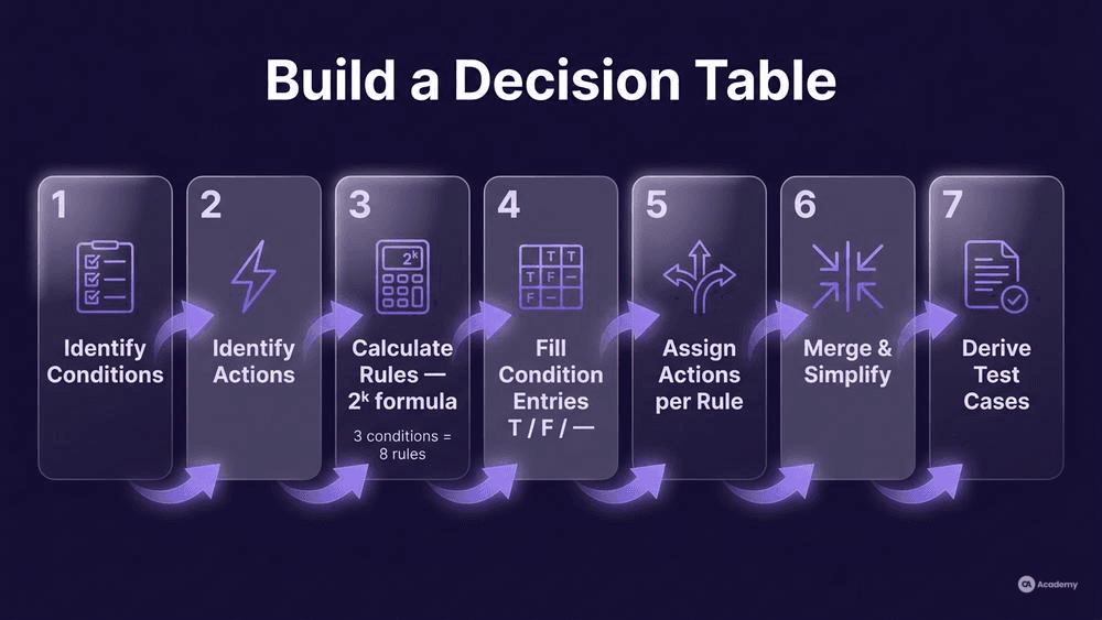
Step 4 — Fill in the Condition Entries
Write out every combination systematically. The simplest pattern: alternate T/F for the last condition every column, every two columns for the second-to-last, and so on — the same pattern used in truth tables.
Step 5 — Assign Actions to Each Rule
For each column, determine which actions fire. This is where you catch contradictions: if two rules produce conflicting actions, the requirement is ambiguous and needs clarification before you write a single test case.
Step 6 — Simplify by Merging Rules
Look for adjacent rules that trigger the same set of actions and differ in only one condition. Replace the differing condition's entry with "—" (don't care) and merge the two columns into one. Repeat until no further merges are possible.
Example: If rules 3 and 4 both produce "Deny access" and differ only in "Has coupon? (T vs. F)," merge them into one rule where "Has coupon?" is marked "—."
Step 7 — Derive Test Cases
Each remaining rule becomes one test case (or more, if boundary values within a condition need separate coverage). Map the test case back to the rule number for traceability.
Common Pitfalls During Construction
- Treating dependent conditions as independent. If Condition B can only be True when Condition A is True, the pair is constrained. The unconstrained table will include impossible rules (A = False, B = True). Mark these as infeasible and remove them — do not simply ignore them, because silent removal hides assumptions.
- Forgetting the "all False" rule. The combination where every condition is False often represents the default or error path. It is easy to overlook and frequently reveals missing requirements.
- Letting the table go stale. A decision table that no longer matches the current logic can be detrimental — it risks giving false confidence that coverage is complete while the logic underneath has shifted. Treat the table as a living artifact: update it when requirements change.
Best Practices for Effective Decision Tables
These practices come from the intersection of ISO/IEC/IEEE 29119-4's formalized technique descriptions [2], the ISTQB syllabus's guidance on test design [1], and Copeland's practical heuristics for black-box techniques [3].
1. Keep each table to one decision. If a requirement contains two independent business decisions, use two tables. A single table that mixes unrelated logic grows exponentially and becomes unreadable.
2. Name conditions and actions in business language. "CND_04 = T" means nothing in a review meeting. "Subscription expired? = Yes" does. Myers, Badgett, and Sandler emphasize that the value of a decision table partly depends on its ability to communicate logic to non-technical stakeholders [4].
3. Validate with stakeholders before deriving tests. The table is a model of the requirement. If the model is wrong, every test case derived from it is wrong too. A 15-minute review session can prevent hours of rework.
4. Automate the mapping where possible. If your test management tool supports parameterized tests, each rule can feed directly into an automated test as a data row. This collapses the gap between design and execution.
5. Version-control the table alongside the requirement. When the requirement changes, diff the table. New conditions add columns; removed conditions delete them. The change is visible and auditable.
What Not to Do — Anti-Patterns and Pitfalls
Do not skip simplification and test every raw combination blindly. For six binary conditions, the full table has 64 rules. Many will share identical action sets. Testing all 64 wastes execution time without adding coverage.
Do not use decision tables for purely sequential logic. If the system's behavior depends on the order of inputs rather than their combination, a state transition diagram is a better fit. Decision tables assume the conditions are evaluated together, not in sequence.
Do not treat "don't care" as "not tested." A "—" entry means the condition's value does not affect the outcome for that rule — so any value is acceptable. It does not mean you skip the condition during execution. Pick a concrete value (True or False) and document your choice.
Do not ignore constraints between conditions. If two conditions are mutually exclusive (e.g., "Payment = Credit Card" and "Payment = Bank Transfer"), the table should not contain a rule where both are True. Mark such combinations as infeasible explicitly; silent omission hides assumptions from reviewers.
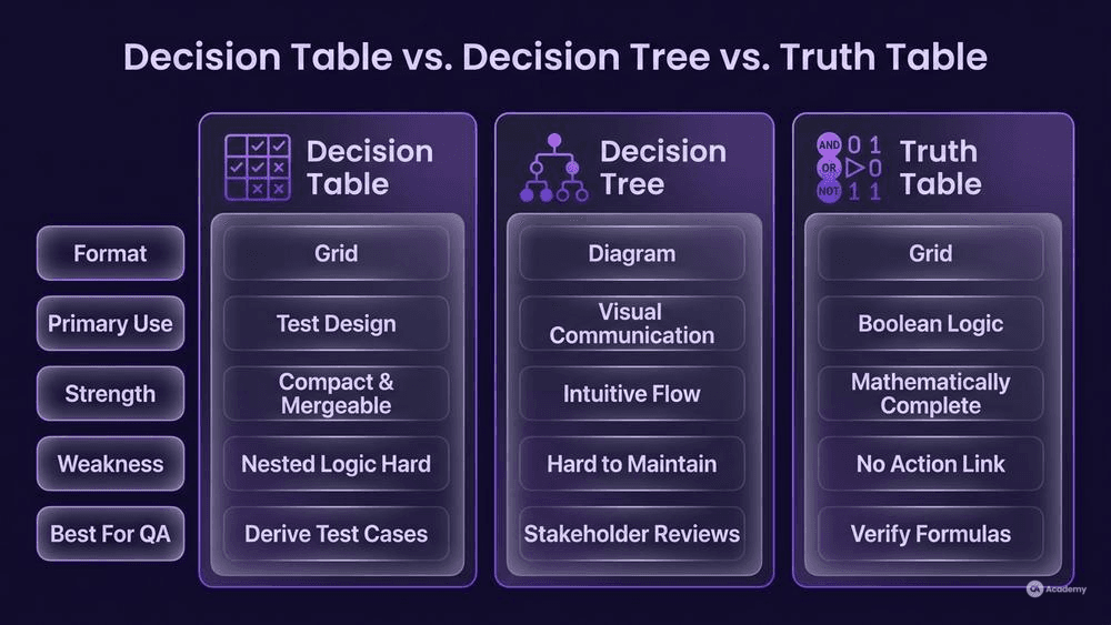
Decision Table vs. Decision Tree vs. Truth Table
Each technique represents conditional logic, but they serve different purposes and audiences. The comparison below summarizes when each is most effective.
Aspect | Decision Table | Decision Tree | Truth Table |
|---|---|---|---|
Format | Grid (rows × columns) | Hierarchical diagram (nodes and branches) | Grid (similar to decision table but logic-focused) |
Primary use | Test design — deriving test cases from business rules | Visual communication — showing decision flow to stakeholders | Formal logic — evaluating Boolean expressions |
Strength | Compact, easy to merge and simplify | Intuitive for non-technical reviewers | Mathematically complete for Boolean analysis |
Weakness | Less intuitive for deeply nested logic | Hard to maintain when conditions change (branches restructure) | No direct link to system actions — purely logical |
Best for QA when | You need to derive test cases and verify completeness | You need to explain logic during a review or walkthrough | You need to verify a Boolean formula or identify redundant conditions |
Decision tree conversion is straightforward: each path from root to leaf in the tree corresponds to one rule in the table. If you inherit a decision tree from a business analyst, converting it to a table lets you check for missing paths — the tree may not show all branches explicitly, but the table's 2^k structure forces you to account for every combination. Copeland describes this conversion process as a practical way to validate that a tree is complete [3].
A truth table comparison is useful when you suspect the conditions contain logical redundancy. If two conditions always have the same truth value, the truth table reveals this and you can eliminate one.
Real-World Example
⚠️ Disclaimer: The following scenario is an illustrative example based on typical industry patterns. The specific metrics are hypothetical estimates designed to demonstrate realistic outcomes, not measured data from a documented project. They should not be cited as factual benchmarks.
Context
A mid-size fintech team handles loan approval logic. The approval depends on four binary conditions: credit score above threshold, employment verified, debt-to-income ratio acceptable, and no active fraud flag. The full rule set is 2^4 = 16 combinations.
Challenge
The team was writing test cases from user stories without a systematic structure. After two releases, production defects showed up in edge-case combinations — specifically, cases where the credit score was above threshold but the fraud flag was active. Testers had assumed that a passing credit score meant approval, without considering the fraud flag interaction.
Solution
The team built a decision table with the four conditions as condition stubs and three actions as action stubs: "Approve loan," "Reject loan," and "Flag for manual review." They followed the step-by-step workflow described above:
- Listed the four conditions and verified their independence with the product owner.
- Generated all 16 rules.
- Assigned actions — discovering two rules where the expected action was genuinely ambiguous (the product owner had not considered the combination of acceptable debt-to-income with an active fraud flag). This triggered a requirements clarification.
- Simplified the table from 16 to 10 rules by merging rules with identical action sets.
- Derived 10 test cases, each traceable to a specific rule.
Results (Illustrative)
After adopting the decision table approach for this module:
- Edge-case defects in the loan approval flow dropped by roughly 70% over the following two release cycles.
- The requirements clarification caught two contradictory business rules before development, avoiding rework.
- Test design time for the module decreased by approximately 55% compared to the previous ad-hoc approach, because the systematic structure eliminated guesswork about which combinations to cover.
Key Takeaways
- The table's structure exposed ambiguous requirements that unstructured test lists had missed.
- Simplification from 16 to 10 rules cut execution time without reducing logical coverage.
- Anchoring each test case to a rule number made traceability audits straightforward.